The Data View is used to display multiple types of information in a variety of formats. Most of the time this will be used for viewing images, especially when navigating through Image Thumbnails or in Merge mode. The information on this section focuses on the organization of measured data and the viewing options provided through the Data Tree. The views are enabled or disabled depending on whether the view type is compatible with the type of data contained in the currently selected node in the Data Tree.
In addition to the same views available from an image document, a data document's fields can also be viewed as a Montage. The Montage can be setup to create 1, 2 or 3-dimensional views of all, or a selected portions of the image data in the file, see "Montage.".
The Data Document file can contain a variety of different Data Types. Each Data Type can be displayed in one or more views, and exported to compatible file formats or to the Windows Clipboard for pasting into other applications for further numerical analysis, report generation or for desktop publishing. The Data Types include:
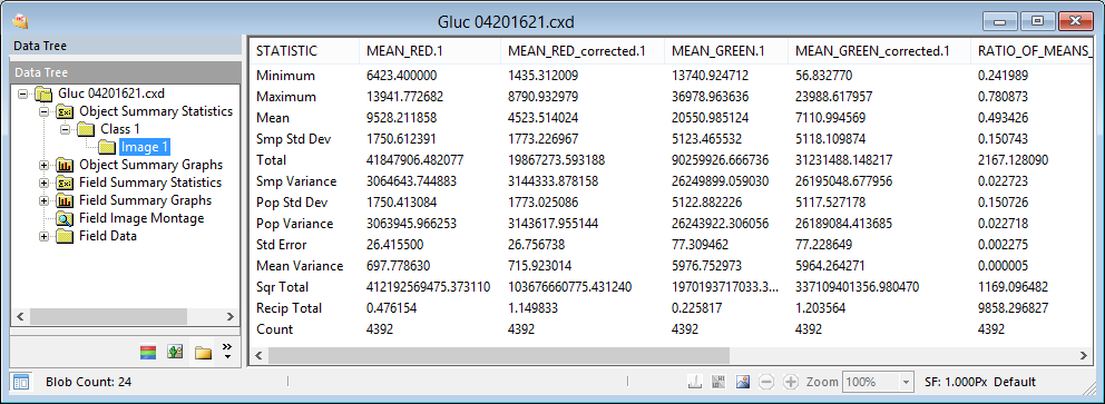
Object Summary Statistics are collected for each of the Object Measurements made for each Measurement Class. As Object Measurements in a Workfile may be selected and deselected during data collection the Count value may vary between Field Measurements. Each Statistic is computed according to the actual Count of Objects processed for each measurement selected.

The Statistics computed for Object and Field Measurements are derived as follows:
Statistic |
Note |
Formula |
|---|---|---|
|
total number of items considered in the data set |
Count = N |
|
|
Minimum |
minimum occurring value in the data set |
Min (x) |
|
Maximum |
maximum occurring value in the data set |
Max (x) |
|
sum of all values in the data set |
Total value = (Σx) |
|
|
Mean |
total value divided by count of items |
µ = (Σx)/N |
|
used to characterize incomplete samples |
s² = (Σx² - (Σx)²/N)/(N-1) |
|
|
used to characterize incomplete samples |
s = √(s² ) |
|
|
used to characterize complete samples |
σ² = (Σx² - (Σx)²/N)/N |
|
|
used to characterize complete samples |
σ = √(σ² ) |
|
|
experimental uncertainty of an averaged measurement |
SEµ = s / √N |
|
|
Total of Values Squared |
sum of squares |
Σx² |
|
Total of Reciprocal Values |
sum of reciprocals |
Σ1/x |
Further statistics can be derived by combining measurement statistics and partial statistics using Custom Measurements.
Object Measurements can be plotted for each object in the data document. The Object Summary Graphs show Object Measurement data of all fields. The interactive graph lets the user customize the display. Use the graph toolbar to select the measurements and which class and objects to display. Use the right-click menu to customize the look and feel of the graph by changing the title and legend fonts or adjusting background and border colors. The right-click menu also allows users to display the X axis as number of fields or field time.
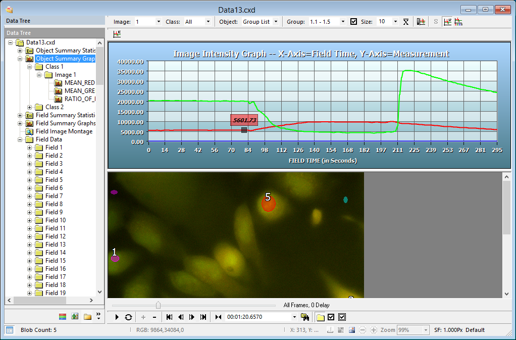
The toolbar provides multiple options for managing how the data is displayed.

Select which image to graph when acquiring multiple monochrome images.
If multiple classes have been identified, use the drop-menu to select one. The Count box displays the total number of objects in the selected class. Select which object(s) to view on the graph using the Object selection box. The option to select all objects or the average of the objects is also available.
The Object list provides multiple options for determining which object(s) will plotted on the graphs.
Define group settings according to:
All of the selected measurements from the Select Intensity Measurements dialog are available in View Measurements. By default only the measurements that were displayed in the graphs when the data was acquired are selected. To add or remove measurements from the graph, click the Select Measurements icon, enable (with a check mark) or disable (no check mark) specific measurements and click OK.
In addition to selecting which measurements will be displayed, the user has the option to select the type of object data to display on the graph. Use the right-click menu and select Show raw and/or corrected data.
This will display the value for the measured object data when hovering the mouse at time points along the graph.
To display or hide the legend, click the Show Legend icon.
Note: Depending on the number of objects and measurements selected, the graph and legend will become very crowded and it may become hard to differentiate the objects. If the number of objects and measurements is too large to properly display in the legend, then the legend will be hidden.
Field Summary Statistics are collected for each of the Field Measurements made for each Measurement Class. As Field Measurements in a Workfile may be selected and deselected during data collection the Count value may vary between Field Measurements. Each Statistic is computed according to the actual Count of Fields processed for each measurement selected.
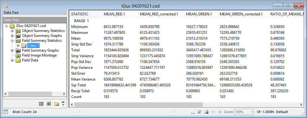
Opening the Field Summary Statistics node will display a node for each Measurement Class present. Selecting the Field Summary Statistics node will display all Field Measurement Classes. Under the Field Summary Statistics node is a node for each Measurement Class. Selecting the Class node will display the Field Measurement Data for the individual Class.
Field Measurements can be plotted for each Field in the Data Document. The Field Summary Graphs show Field Measurement parameters for each Measurement Class with the Field number as the X axis variable and the Field Measurement as the Y axis variable.
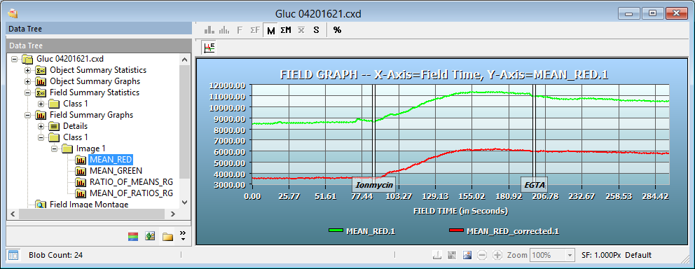
The Field Summary graphs are an easy to use interactive way of displaying and viewing data. First the Mean Red (Corrected 340nm) Intensity is measured over Time. Second there are three Event Markers that indicate specific points during the experiment that an event happened. In this case, we know the name and the amount of the reagents that were added and the time they were added. The Event Markers may be toggled on and off by clicking the Show Event Markers Icon ( ). The intensity at any given point is displayed by hovering the cursor over a section of the graph. The corresponding image may also be viewed by clicking on a point along the graph. Zoom in on a specific area of the graph by clicking and dragging the mouse over the area of interest. Use the playback functions located on the Playback Toolbar to watch the intensity changes of the sample. Using the features in the Playback Toolbar we can play the image sequence and visually see the changes in the intensity and how they are plotted on the corresponding graph. Use the right-click menu to customize the look and feel of the graph by changing the title and legend fonts or adjusting background and border colors. The right-click menu also allows users to display the X axis as number of fields or field time.
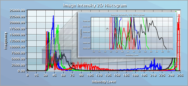
To zoom in on a particular area click and hold the left mouse button as you drag a box around the area of interest. Release the button and the graph zooms to the size of the box. Click the left mouse button to return to the normal view. While in a zoomed position the user can pan by dragging the mouse in the direction they wish to view. In the example below, a portion of a 2-D Histogram has been enlarged.
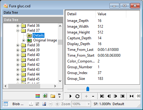
The Field Details node contains information for each field about when and where the image was captured. The Field Details can be viewed in a Table View or Spreadsheet View and copied to the Windows Clipboard, or in Graphical form.
These details can include:
Object Measurement data are collected for each of the Object Measurements selected for each Measurement Class. They can be viewed from the Object Data node of each Field. Object Statistics and Object Graphs are also available for each field of data measured.
